5. Improvements and new features available in Algotom
Sarepy is actually a part of the Algotom package which was released first to support the paper in Ref. [1]. Sarepy wasn’t packaged. From 05/2021, it were integrated into Algotom with improvements to be more flexible and easy-to-maintain. There are many utility methods allowing users to customize their own ring removal methods. This section demonstrates these new features related to ring removal methods in Algotom.
5.1. Improvements
Users can select different smoothing filters (in scipy.ndimage or algotom.util.utility) for cleaning stripes by passing keyword arguments as dict type:
import algotom.io.loadersaver as losa
import algotom.prep.removal as rem
sinogram = losa.load_image("D:/data/sinogram.tif")
# Sorting-based methods use the median filter by default, users can select
# another filter as below.
sinogram1 = rem.remove_stripe_based_sorting(sinogram,
                                           option={"method": "gaussian_filter",
                                                   "para1": (1, 21)})
The sorting-based technique, which is simple but effective to remove partial stripes and avoid void-center artifacts, is an option for other ring removal methods.
sinogram2 = rem.remove_stripe_based_filtering(sinogram, 3, sort=True)
sinogram3 = rem.remove_stripe_based_regularization(sinogram, 0.005, sort=True)
5.2. Tools for designing ring removal methods
The cleaning capability with least side-effect of a ring removal method relies on a smoothing filter or an interpolation technique which the method employs. Other supporting techniques for revealing stripe artifacts such as sorting, filtering, fitting, wavelet decomposition, polar transformation, or forward projection are commonly used. Algotom provides these supporting tools for users to incorporate with their own smoothing filters or interpolation techniques.
5.2.1. Back-and-forth sorting
The technique (algorithm 3) couples an image with an index array for sorting the image backward and forward along an axis. Users can combine the sorting forward method, a customized filter, and the sorting backward method as follows
import algotom.util.utility as util
import scipy.ndimage as ndi

# Sort forward
sino_sort, mat_index = util.sort_forward(sinogram, axis=0)
# Use a customized smoothing filter here
sino_sort = apply_customized_filter(sino_sort, parameters)
# Sort backward
sino_corr = util.sort_backward(sino_sort, mat_index, axis=0)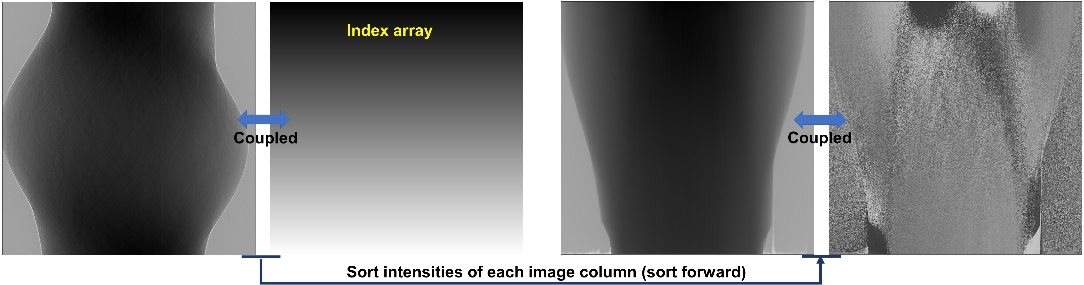
Figure 1. Demonstration of the forward sorting.
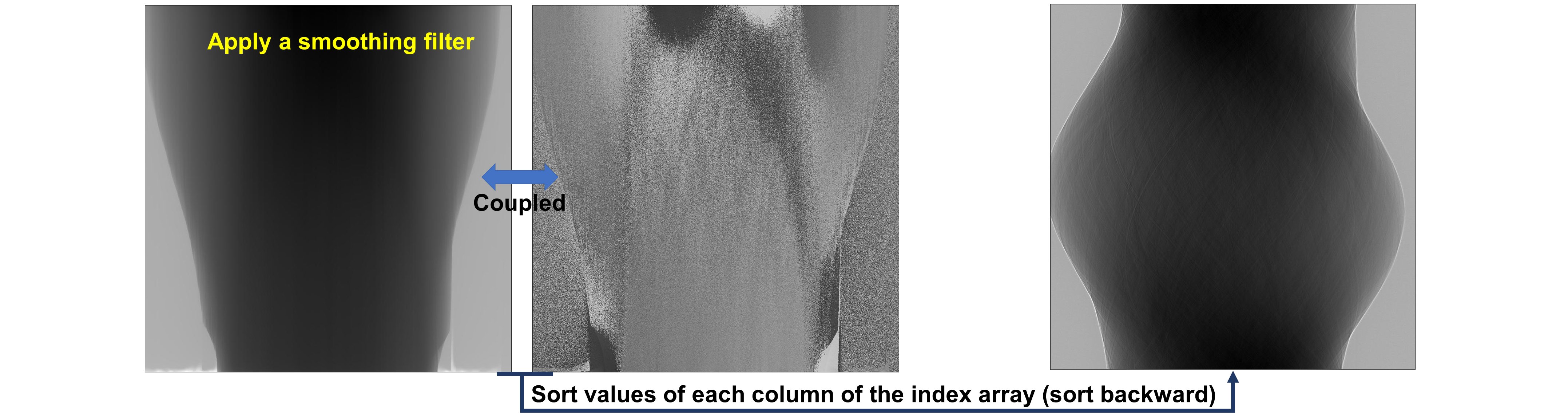
Figure 2. Demonstration of the backward sorting.
5.2.2. Separation of frequency components
The technique can help to reveal stripe artifacts by separating frequency components of each image-column using a 1D window available in Scipy. Example of how to use the technique:
sino_smooth, sino_sharp = util.separate_frequency_component(sinogram, axis=0,
                                                            window={"name": "gaussian",
                                                                    "sigma": 5})
# Use a customized smoothing filter here
sino_smooth = apply_customized_filter(sino_smooth, parameters)
sino_corr = sino_smooth + sino_sharp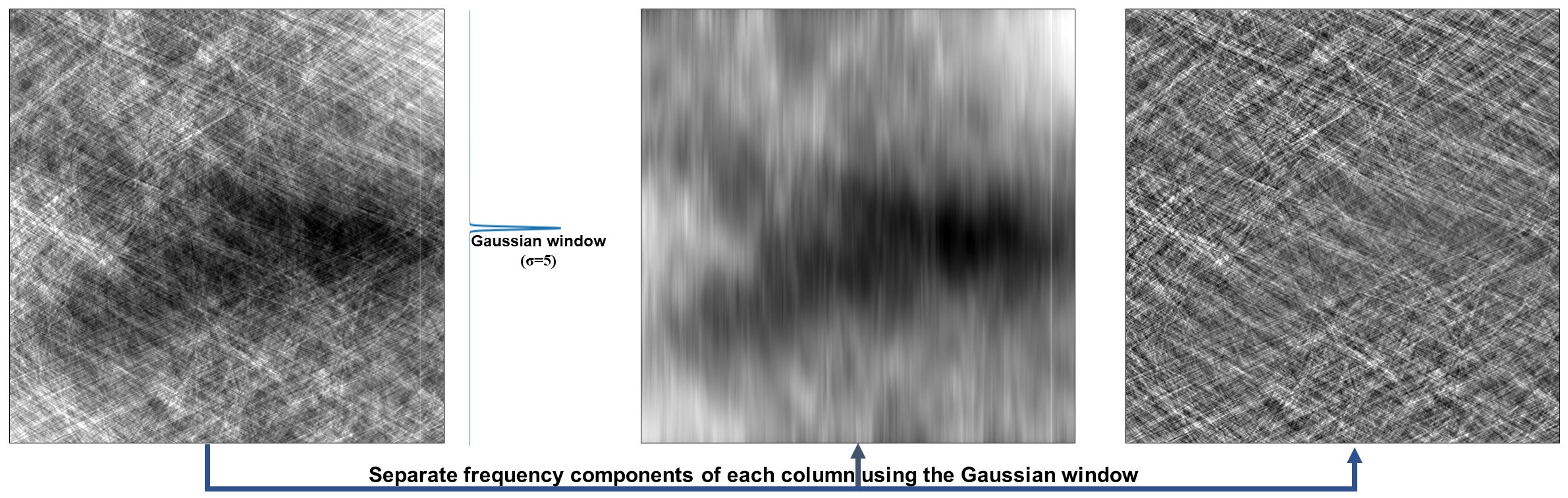
Figure 3. Demonstration of how to separate frequency components of a sinogram along each column.
5.2.3. Polynomial fitting along an axis
The technique can help to reveal low contrast stripes easily by applying a polynomial fit along each image-column.
sino_fit = util.generate_fitted_image(sinogram, 3, axis=0, num_chunk=1)
# Use a customized smoothing filter here
sino_smooth = apply_customized_filter(sino_fit, parameters)
sino_corr = (sinogram / sino_fit) * sino_smooth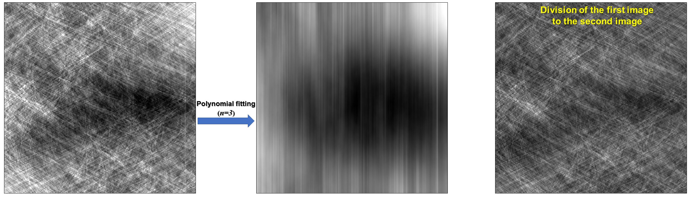
Figure 4. Demonstration of how to apply a polynomial fitting along each column of a sinogram.
5.2.4. Wavelet decomposition and reconstruction
Functions for wavelet decomposition, wavelet reconstruction, and applying a smoothing filter to specific levels of directional image-details are provided. The following codes decompose a sinogram to level 2. As can be seen in Fig. 5 stripe artifacts are visible in vertical details of results. One can apply a smoothing filter to remove these stripes then apply a wavelet reconstruction to get the resulting sinogram.
outputs = util.apply_wavelet_decomposition(sinogram, "db9", level=2)
[mat_2, (cH_level_2, cV_level_2, cD_level_2), (cH_level_1, cV_level_1, cD_level_1)] = outputs
# Save results of vertical details
# losa.save_image("D:/tmp/output/cV_level_2.tif", cV_level_2)
# losa.save_image("D:/tmp/output/cV_level_1.tif", cV_level_1)
# Apply the gaussian filter to each level of vertical details
outputs = util.apply_filter_to_wavelet_component(outputs, level=None, order=1,
                                                 method="gaussian_filter", para=[(1, 11)])
# Optional: remove stripes on the approximation image (mat_2 above)
outputs[0] = rem.remove_stripe_based_sorting(outputs[0], 11)
# Apply the wavelet reconstruction
sino_corr = util.apply_wavelet_reconstruction(outputs, "db9")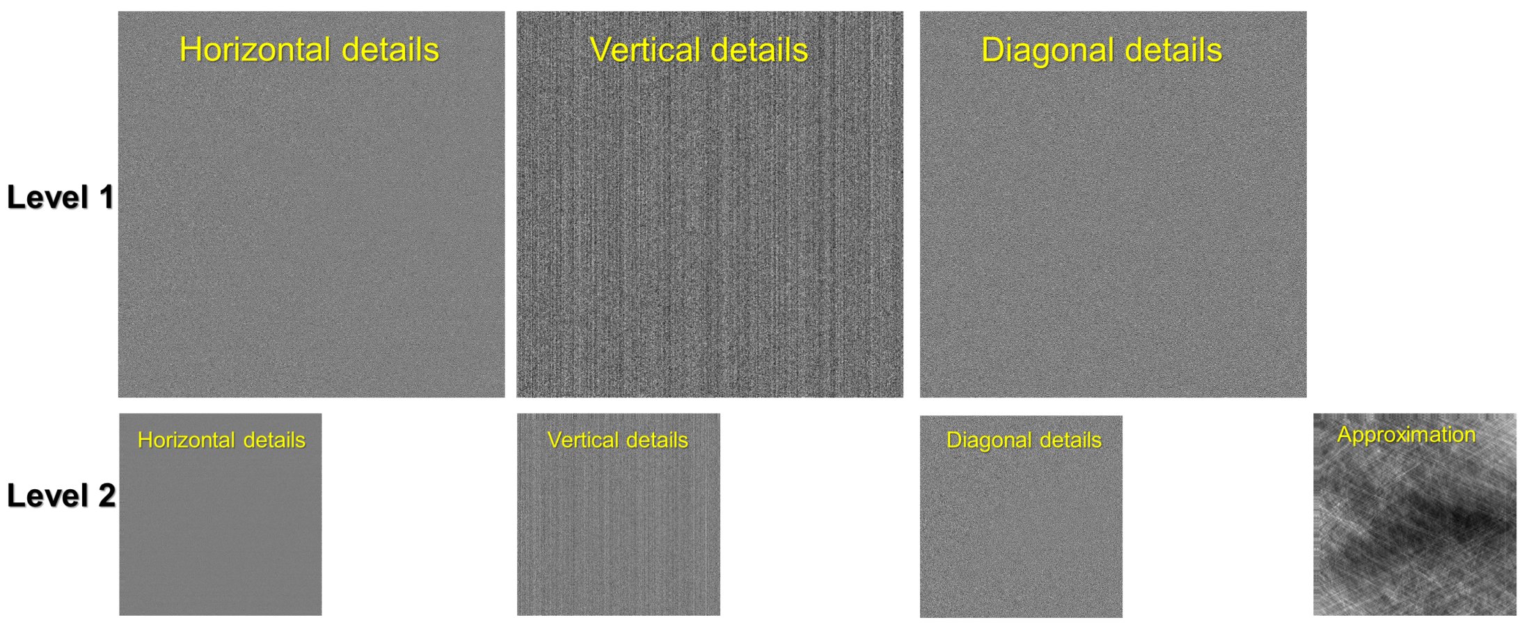
Figure 5. Demonstration of the wavelet decomposition.
5.2.5. Stripe interpolation
Users can design a customized stripe-detection method, then pass the result (as a 1D binary array) to the following function to remove stripes by interpolation.
sino_corr = util.interpolate_inside_stripe(sinogram, list_mask, kind="linear")
5.2.6. Transformation between Cartesian and polar coordinate system
This is a well-known technique to remove ring artifacts from a reconstructed image as shown in section 3.2.
img_rec = losa.load_image("D:/data/reconstructed_image.tif")
# Transform the reconstructed image into polar coordinates
img_polar = util.transform_slice_forward(img_rec)
# Use a customized smoothing filter here
img_corr = apply_customized_filter(img_polar, parameters)
# Transform the resulting image into Cartesian coordinates
img_carte = util.transform_slice_backward(img_corr)
5.2.7. Transformation between sinogram space and reconstruction space
Algotom provides a re-projection method to convert a reconstructed image to the sinogram image. As using directly the Fourier slice theorem it’s fast compared to ray-tracing-based methods or image-rotation-based methods.
import numpy as np
import algotom.util.simulation as sim
import algotom.rec.reconstruction as rec

rec_img = losa.load_image("D:/data/reconstructed_image.tif")
(height, width) = rec_img.shape
angles = np.deg2rad(np.linspace(0.0, 180.0, height))
# Re-project the reconstructed image
sino_calc = sim.make_sinogram(rec_img, angles=angles)
# Use a customized stripe-removal method
sino_corr = apply_customized_filter(sino_calc, parameters)
# Reconstruct
img_rec = rec.dfi_reconstruction(sino_corr, (width - 1) / 2, apply_log=False)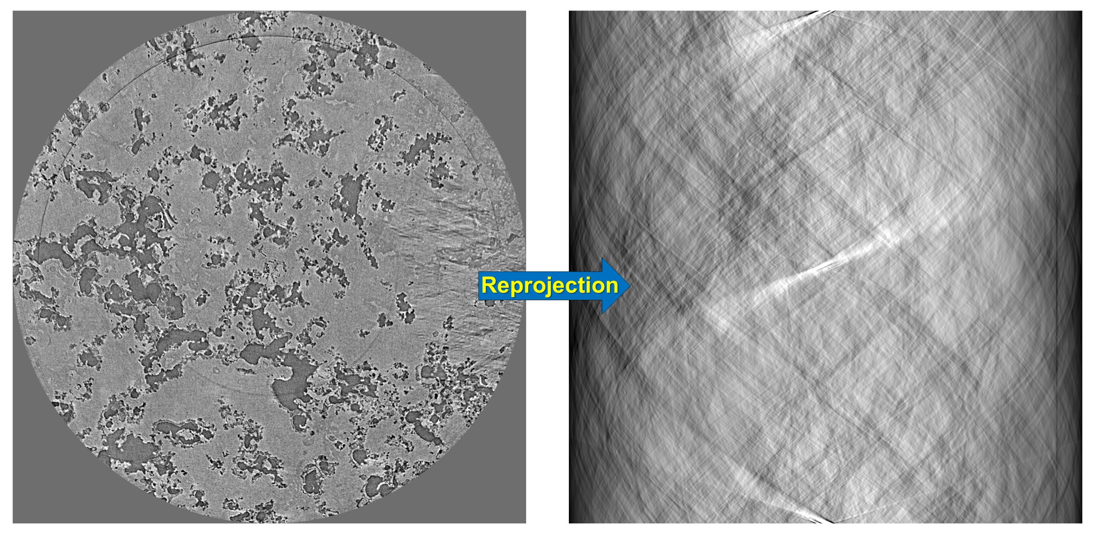
Figure 6. Demonstration of how to re-project a reconstructed image.