3.1.1. Equalization-based methods for removing partial and full stripe artifacts
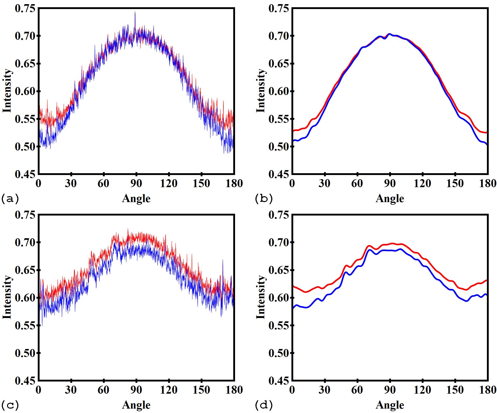
Figure 1. Characteristic intensity profile of a defective pixel (red color) in comparison with an adjacent good pixel (blue color). (a) Partial stripe. (b) Low-pass filter of the intensities in (a). (c) Full stripe. (d) Low-pass filter of the intensities in (c)
As can be seen in Fig.1, the differences in low-frequency components between the intensity profiles of adjacent pixels causes stripe artifacts. To remove stripes, we need to equalize the responses of these pixels. This can be done by applying a smoothing filter along the horizontal direction of a sinogram. This approach, however, introduces void-center artifacts and blurs reconstructed image. To workaround these problems, a sinogram can be transformed or pre-processed to reveal underlying response curves, then a smoothing filter or a correction method can be applied. There are 3 different ways of extracting the underlying responses as shown below; ordered from fine to coarse extraction.
3.1.1.1. Sorting-based approach
Code
- sarepy.prep.stripe_removal_original.remove_stripe_based_sorting(sinogram, size, dim=1)[source]
Remove stripe artifacts in a sinogram using the sorting technique, algorithm 3 in Ref. [1]. Angular direction is along the axis 0.
- Parameters
sinogram (array_like) – 2D array. Sinogram image.
size (int) – Window size of the median filter.
dim ({1, 2}, optional) – Dimension of the window.
- Returns
ndarray – 2D array. Stripe-removed sinogram.
References
How it works
This is a very simple but efficient method. It retrieves the response of each pixel by sorting intensities along each column of a sinogram. Then, the median filter is applied along the horizontal direction to remove stripes. The resulting image is re-sorted to get back the sinogram image. This approach can be explained using the following approximating assumptions: adjacent areas of a detector system are sampling the same range of incoming flux because a sample has continuous variation in intensity; irregular areas are small compared to the representative level of details in the sample. If the detector system is ideal, the total range of brightness observed at neighboring pixels should be the same.
This means that if the measured intensities are sorted in order of brightness, we should expect the same distribution in neighboring pixels. Under the assumption of small irregular areas, we can use the brightness sorted values to identify, compare and correct the irregular areas. Applying a smoothing filter is the easiest way of correction. To transform back and forth between the normal sinogram and the sorted sinogram, the intensities in each column are coupled with their indexes. This is a very handy technique and can be useful elsewhere. The visual explanation of the method is as follows (use the browser zoom to see the details).
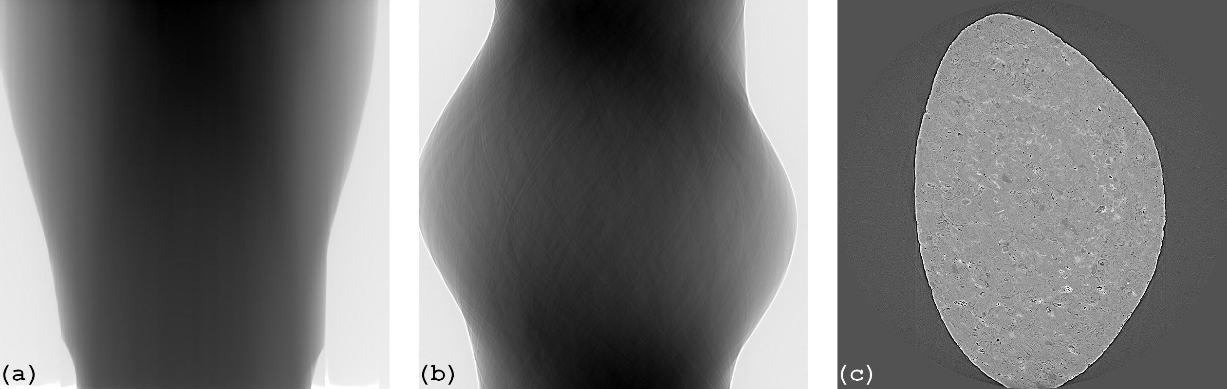
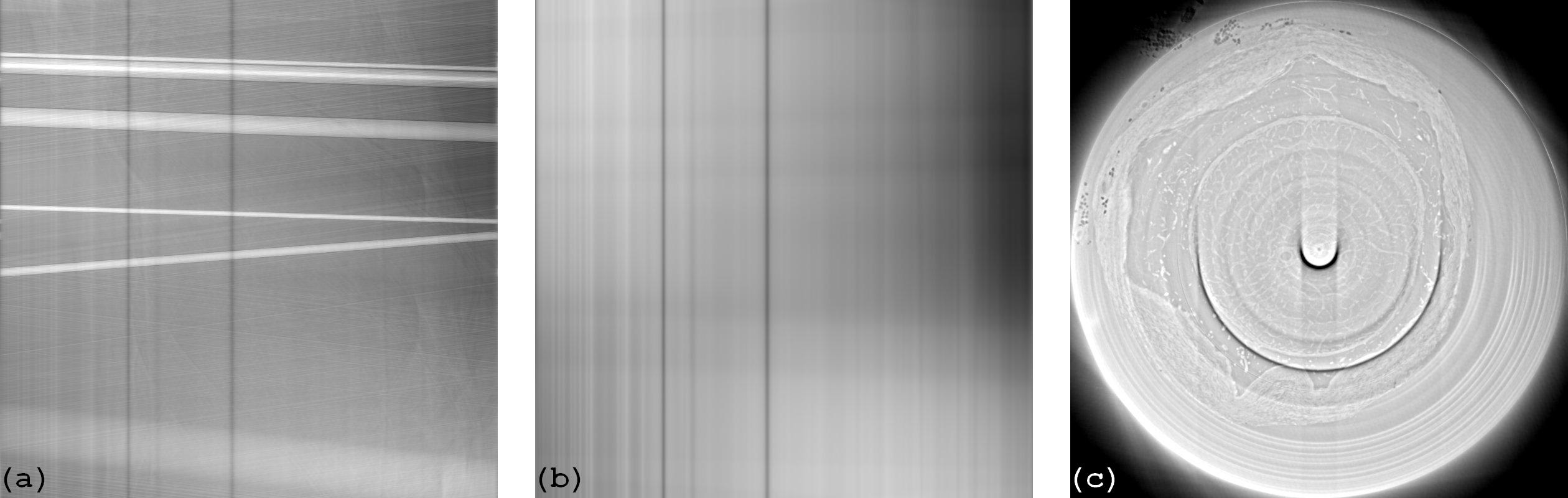
Step 1. Original sinogram (a) is coupled with an index matrix (b). (c) is the reconstructed image from (a).
Step 2. Intensities of each column are sorted (a). The index matrix is changed correspondingly (b).
Step 3. Sorted image is smoothed along the horizontal direction (a). Corrected sinogram (b) is re-sorted using the index matrix in the previous step. (c) is the reconstructed image from (b).
How to use
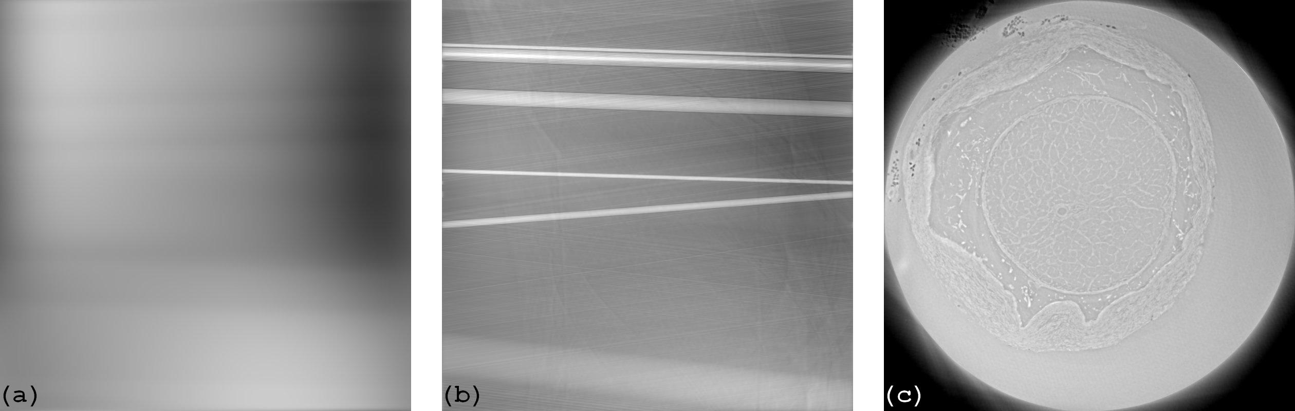
Users adjust the size of the median filter to adjust the strength of the method. Larger is stronger. A practical rule is that it should be larger than the largest size of stripes, but not too large to increase side-effect artifacts, which are streak artifacts (Fig. 2). The tolerance range of the window size depends on the complexity of features of a sorted sinogram (Step 2(a)). In most cases, it’s pretty simple. This means that we can use the same size across sinograms of a 3D tomographic data.
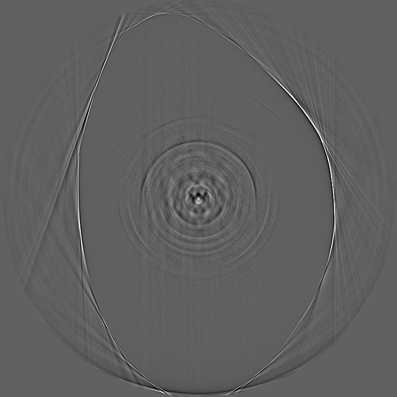
Figure 2. Difference in the reconstruction space between the corrected sinogram using the size of 71 and the one using the size of 31 (not much different if using 30 or 32). Sinograms for testing are available here.
Users can choose to apply a 1D smoothing filter or 2D smoothing filter using the dim parameter. However, the 1D filter is good enough for most cases.
Pros
– It is very simple to use and works particularly well to remove partial stripes.
– It does not yield extra stripe artifacts and void-center artifacts.
– Fixed parameters can be used for full datasets.Cons
– It can introduce streak artifacts.
– The method uses the whole range of intensities for sorting while it is the low-pass components need to be corrected. This means that if the ratio of the high-pass components is high (e.g noisy data) it can alter the sorting order which results streak artifacts.
– It won’t work well on synthetic stripes, stripes introduced by tomographic alignment, or any stripes where rankings of intensities are significantly different between pixels inside stripes and outside stripes.How to improve
– The median filter, an edge-preserving smoothing filter, is used to reduce the side effect of introducing streak artifacts. However, for sinograms without sharp jumps of intensities between columns, other types of smoothing filters, which are stronger and faster, can be used (Fig. 3). This can be useful to remove the low-frequency ring artifacts in a low-contrast reconstructed image.
– The smoothing filter is not applied to a small percentage of pixels at the top and bottom of a sorted sinogram. This can reduce streak artifacts.
– The method can be used only to the low-pass components of sinogram columns by combing with the filtering-based approach as will be shown below.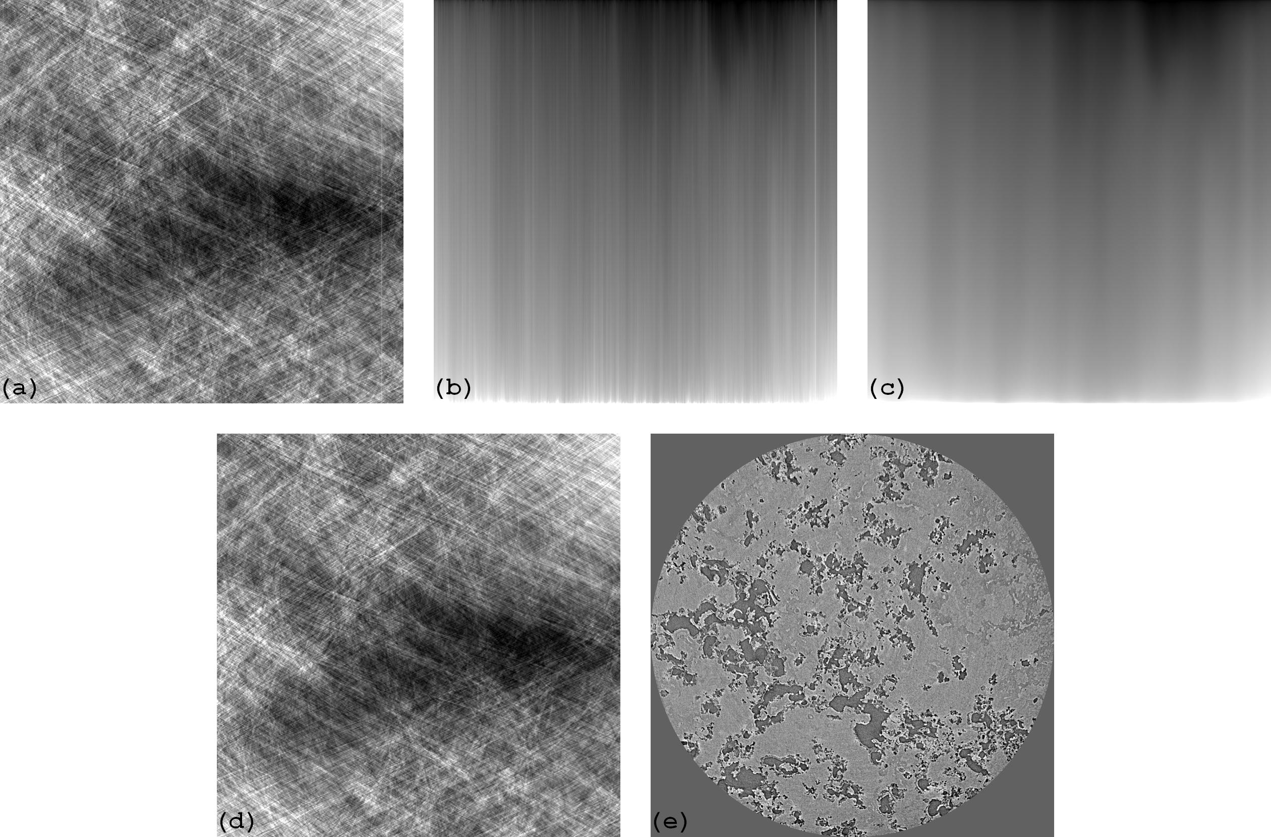
Figure 3. Results of the sorting-based approach where the gaussian filter with the sigma of 31 is used instead of the median filter. (a) Original sinogram. (b) Sorted sinogram. (c) Smoothing of the sorted sinogram. (d) Corrected sinogram. (e) Reconstructed image.
3.1.1.2. Filtering-based approach
Code
- sarepy.prep.stripe_removal_original.remove_stripe_based_filtering(sinogram, sigma, size, dim=1)[source]
Remove stripe artifacts in a sinogram using the filtering technique, algorithm 2 in Ref. [1]. Angular direction is along the axis 0.
- Parameters
sinogram (array_like) – 2D array. Sinogram image
sigma (int) – Sigma of the Gaussian window used to separate the low-pass and high-pass components of the intensity profile of each column.
size (int) – Window size of the median filter.
dim ({1, 2}, optional) – Dimension of the window.
- Returns
array_like – 2D array. Stripe-removed sinogram.
References
How it works
It uses directly the assumption shown in Fig. 1 by: extracting the low-pass components of each column using the Fourier transform, applying a smoothing filter across columns, combing the result with the high-pass components. The visual explanation of the method is as follows.
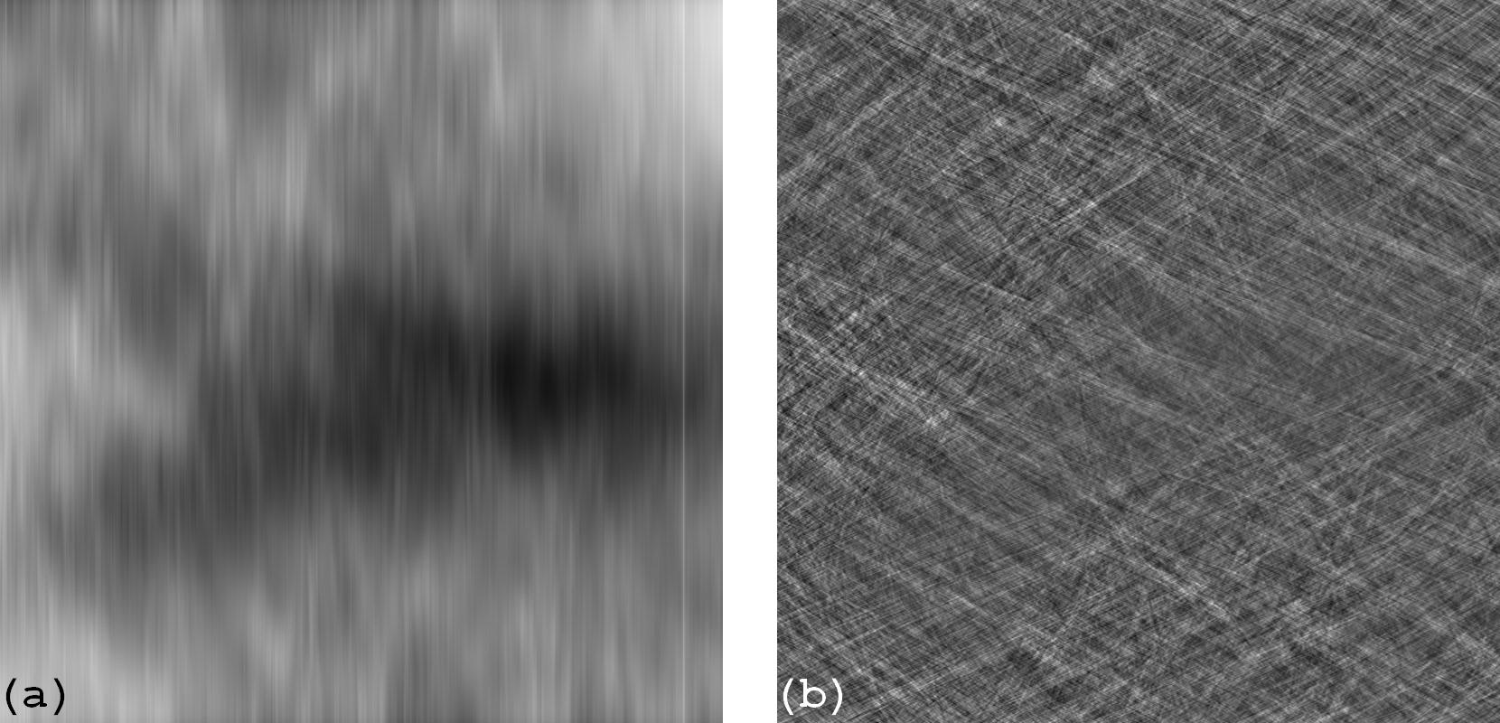
Step 1. Original sinogram (Fig. 3(a)) is separated into the low-pass components (a) and the high-pass components (b).
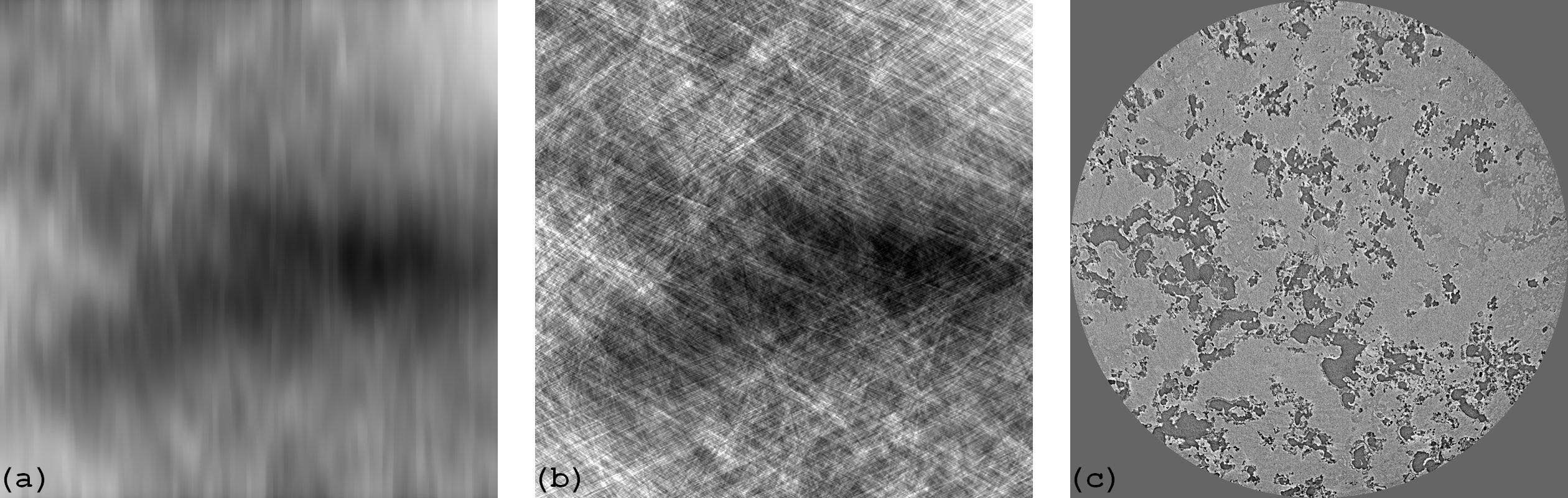
Step 2. (a) Low-pass image is smoothed along the horizontal direction. Corrected sinogram (b) is formed by adding image (a) and the high-pass components (Step 1(b)). (c) is the reconstructed image from (b).
How to use
– The sigma parameter controls the size of the window (in the Fourier space) used for separating the low-pass components and the high-pass components. It should be chosen in the range of (0 -> 10) as higher values give rise to void-center artifacts.
– The size parameter controls the strength of the median filter. Larger is stronger.
– The dim parameter allows to select the 1D or 2D median filter.
Pros
– It is an intuitive method and easy to use.
– It does not yield extra stripe artifacts.
Cons
– It can yield void-center artifacts.
– It can result in streak artifacts.
– It doesn’t work well on sinograms having sharp jumps of intensities between columns, e.g the sinogram used in section 3.1.1.1.
How to improve
– Different windows can be used to separate the low-pass components.
– Can be used with other edge-preserving smoothing filters.
– The problem of yielding void-center artifacts can be solved by combining with the sorting-based method as below.
– Code:
- sarepy.prep.stripe_removal_improved.remove_stripe_based_filtering_sorting(sinogram, sigma, size, dim=1)[source]
Removing stripes using the filtering and sorting technique, combination of algorithm 2 and algorithm 3 in Ref.[1]. Angular direction is along the axis 0.
- Parameters
sinogram (array_like) – 2D array. Sinogram image.
sigma (int) – Sigma of the Gaussian window used to separate the low-pass and high-pass components of the intensity profile of each column.
size (int) – Window size of the median filter.
dim ({1, 2}, optional) – Dimension of the window.
- Returns
ndarray – 2D array. Stripe-removed sinogram.
References
3.1.1.3. Fitting-based approach
Code
- sarepy.prep.stripe_removal_original.remove_stripe_based_fitting(sinogram, order, sigmax, sigmay)[source]
Remove stripes using the fitting technique, algorithm 1 in Ref. [1]. Angular direction is along the axis 0.
- Parameters
sinogram (array_like) – 2D array. Sinogram image
order (int) – Polynomial fit order.
sigmax (int) – Sigma of the Gaussian window in the x-direction.
sigmay (int) – Sigma of the Gaussian window in the y-direction.
- Returns
ndarray – 2D array. Stripe-removed sinogram.
References
How it works
This method is an extreme of the filtering-based method where low-pass components are extracted by applying polynomial fitting in the real space. Because of that it is limited to be used for sinograms having low dynamic range of intensities where its low-pass components can be represented by a low order polynomial fit. Steps of the method are: applying a polynomial fit to each column using the same order resulting the fitted sinogram; applying a smoothing filter along the horizontal direction to remove vertical stripes; multiplying the smoothed sinogram by the original sinogram, then dividing the result by the fitted sinogram. The visual explanation of the steps is as follows.
Step 1. Polynomial fitting is applied to the original sinogram (a) resulting the fitted sinogram (b). (c) is the reconstructed image from (a).
Step 2. Smoothed sinogram (a) is generated by applying the FFT-based smoothing filter to the fitted sinogram. The corrected sinogram is the result of multiplying the original sinogram by the smoothed sinogram then dividing the result by the fitted sinogram. (c) is the reconstructed image from (b).
How to use
– The order parameter allows to select the polynomial order for fitting. It should be chosen in the range of (1->5).
– The sigmax parameter controls the strength of the cleaning capability. Smaller is stronger (as it works in the Fourier space). Recommended values: 2-> 20.
– The sigmay parameter can help to reduce the side effects and is insensitive. Recommended values: 50 -> 200.
Pros
– Powerful method for removing blurry stripes or low-pass stripes.
– Many choices for the smoothing filter.
Cons
– Limited to be used on sinograms having low dynamic range of intensities, i.e. its low-frequency components can be fitted to a low order polynomial.
– Can yield extra stripe artifacts if there are sharp jumps in intensities of each sinogram column.
How to improve
– Can be used with different smoothing filters.
– Can be combined with the sorting-based method to work with more complex sinograms.
– Code:
- sarepy.prep.stripe_removal_improved.remove_stripe_based_sorting_fitting(sinogram, order, sigmax, sigmay)[source]
Remove stripes using the sorting and fitting technique, combination of algorithm 2 and 1 in Ref. [1]. Angular direction is along the axis 0.
- Parameters
sinogram (array_like) – 2D array. Sinogram image.
order (int) – Polynomial fit order.
sigmax (int) – Sigma of the Gaussian window in the x-direction.
sigmay (int) – Sigma of the Gaussian window in the y-direction.
- Returns
ndarray – 2D array. Stripe-removed sinogram.
References