3.1.3. Method for locating stripe artifacts
The techniques described in the previous sections are able to remove full and partial stripe artifacts which are of small or medium size without significantly affecting other areas. However, for large stripes, applying a stronger filter to the whole sinogram will degrade the final image. Furthermore, large stripes are few in number. In this case, the correction could be selectively applied only on defective pixels.
There are other types of stripe artifacts which can’t be removed using the previous approaches such as unresponsive stripes, fluctuating stripes, synthetic stripes, or stripes introduced by tomographic alignment or cone-beam parallel-beam conversion. A practical approach is to locate them first, and then remove them using interpolation methods.
A segmentation algorithm which works on a 1D array to locate stripes was proposed in Ref. [1]. It’s very efficient and simple to use. Depending on the types of stripe artifacts, different pre-processing steps are used to generate an 1D array which then is input to the segmentation algorithm. Steps of this algorithm, called SFTS (Sorting, Fitting, and Thresholding-based Segmentation) for short, is described as follows and demonstrated in Fig. 1.
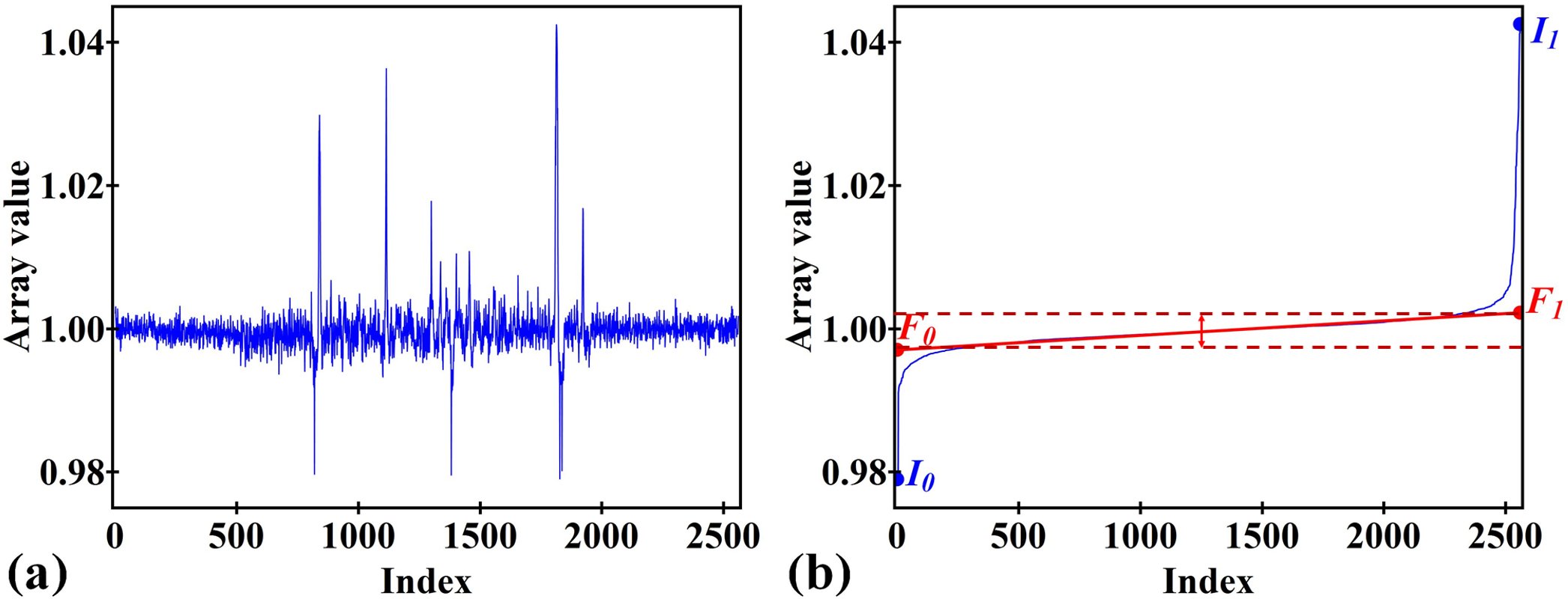
Figure 1. Demonstration of the segmentation algorithm. (a) Normalized 1D array, i.e. non-uniform background is corrected. (b) Sorted array and fitted array using the middle part of the sorted array.
Code
- sarepy.prep.stripe_removal_original.detect_stripe(list_data, snr)[source]
Locate stripe positions using Algorithm 4 in Ref. [1].
- Parameters
list_data (array_like) – 1D array. Normalized data.
snr (float) – Ratio used to segment stripes from background noise.
- Returns
ndarray – 1D binary mask.
References
How it works
As can be seen in Fig. 1(a), it is difficult to segment the array as one doesn’t know which thresholding values should be used. However, if the array values are sorted (Fig. 1(b)), the segmentation task is much easier. If a straight line is drawn along the middle part of the sorted array, it cuts the vertical lines at two points. Vertical distance between these points corresponds to noise level. Values higher than this level at a certain ratio, which is a user-input value, corresponds to stripe locations. Steps of the algorithm are as follows.
Step 1: Sort values of a 1D array into ascending order.
Step 2: Apply a linear fit to the values around the middle of the sorted array, i.e. half of the array size, respect to the array indexes.
Step 3: Calculate the upper threshold, \(T_{U}\), and the lower threshold, \(T_{L}\), using the following formula:
If \((F_{0}-I_{0})/(F_{1}-F_{0})>R,\)
\[T_{L} = F_{0} - (F_{1} - F_{0}) \times R / 2\]If \((I_{1}-F_{1})/(F_{1}-F_{0})>R,\)
\[T_{U} = F_{1} + (F_{1} - F_{0}) \times R / 2\]where \(I_{0}\) and \(I_{1}\) are the minimum and maximum value of the sorted array; \(F_{0}\) and \(F_{1}\) are the fitted value at the first and last index of the array; and \(R\) is a user-input value.
Step 4: Binarize the array by replacing all values between \(T_{L}\) and \(T_{U}\) with 0 and others with 1.