3.1.5. Method for removing unresponsive and fluctuating stripes
Unresponsive and fluctuating stripes give rise to both ring artifacts and streak artifacts in the reconstructed image (Fig. 1). Unfortunately, they cannot be removed using the smoothing-based approaches as in the previous methods because intensity profiles are significantly different between pixels inside stripes and outside stripes. A simple way of removing them is to use an interpolation technique after locating them. The intensity profiles of those stripes show opposite characteristics. The unresponsive stripe shows very little variation while the fluctuating stripe shows excessive variation. Exploiting these features can help us detect them all together.
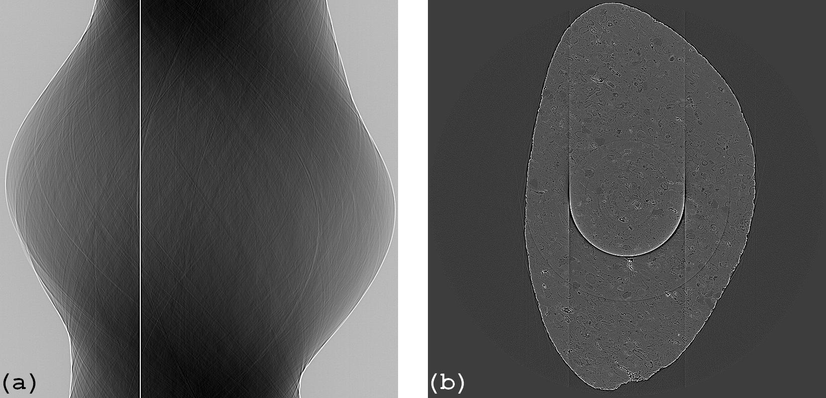
Figure 1. (a) Sinogram with unresponsive stripe artifacts and fluctuating stripe artifacts (zoom-in needed). (b) Reconstructed image.
Code
- sarepy.prep.stripe_removal_original.remove_unresponsive_and_fluctuating_stripe(sinogram, snr, size, residual=False)[source]
Remove unresponsive or fluctuating stripes, algorithm 6 in Ref. [1], by: locating stripes, correcting using interpolation. Angular direction is along the axis 0.
- Parameters
sinogram (array_like) – 2D array. Sinogram image.
snr (float) – Ratio used to segment stripes from background noise.
size (int) – Window size of the median filter.
residual (bool, optional) – Removing residual stripes if True.
- Returns
ndarray – 2D array. Stripe-removed sinogram.
References
How it works
1. Locating stripe artifacts
– Apply the strong mean filter along each column of the sinogram (Fig. 2(a)). Take absolute values of the difference between the result and the original sinogram (Fig. 1(a)) resulting in Fig. 2(b).
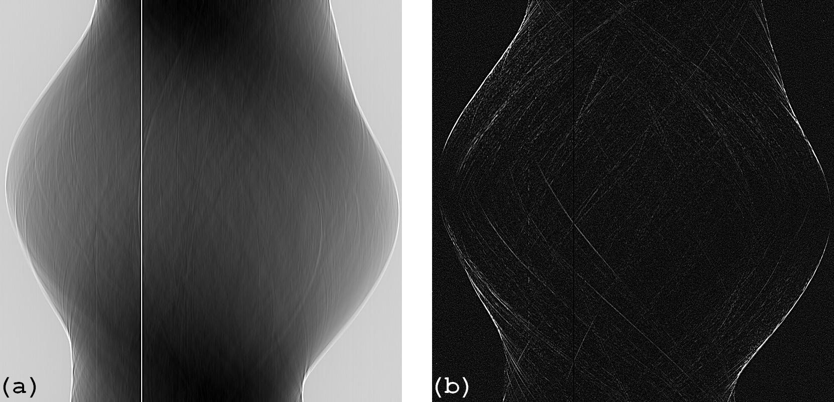
Figure 2. (a) Smoothed sinogram along the verstical direction. (b) Absolute difference between (a) and Fig. 1(a).
—Average along each column of Fig. 2(b) resulting a 1D array (Fig. 3(a)). Apply the strong median filter to this array resulting in Fig. 3(b).
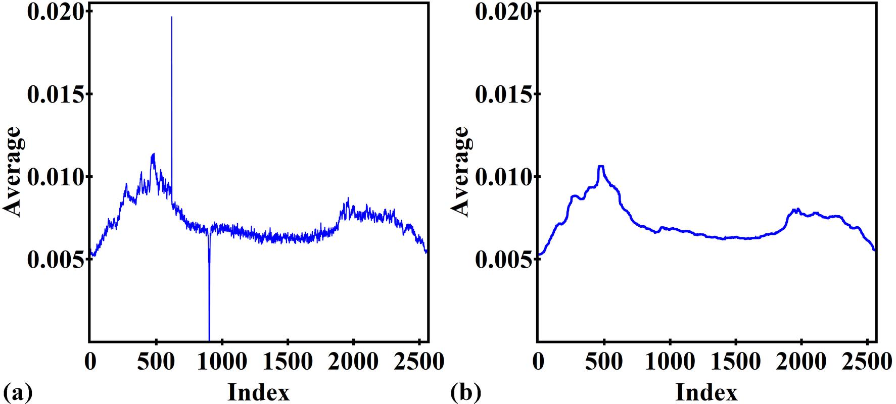
Figure 3. (a) Result of averaging each column of Fig. 2(b). (b) After applying the median filter to (a).
—Divide the result shown in Fig. 3(a) to the result shown in Fig. 3(b) resulting in the normalized 1D array (Fig. 4(a)). Use the SFTS algorithm to get stripe locations (Fig. 4(b)).
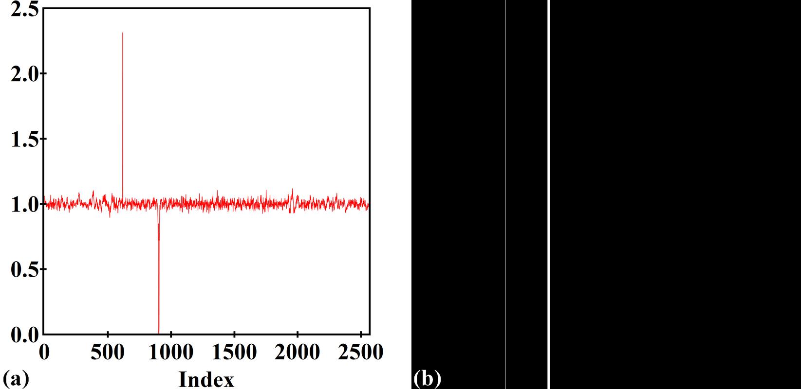
Figure 4. (a) Normalized 1D array used for the SFTS algorithm. (b) Mask indicating the stripe locations.
2. Correcting by interpolation
– Interpolate values inside the stripes from neighboring pixels.
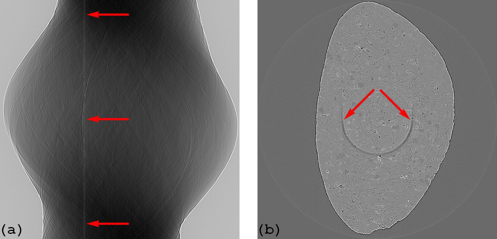
Figure 6. (a) Corrected sinogram. (b) Reconstructed image from sinogram (a).
3. Removing residual stripes (Optional)
– Apply the algorithm of removing large stripes to remove residual stripes. This step may be needed because intensities around dead pixels are modulated by the scattered light resulting large stripes.
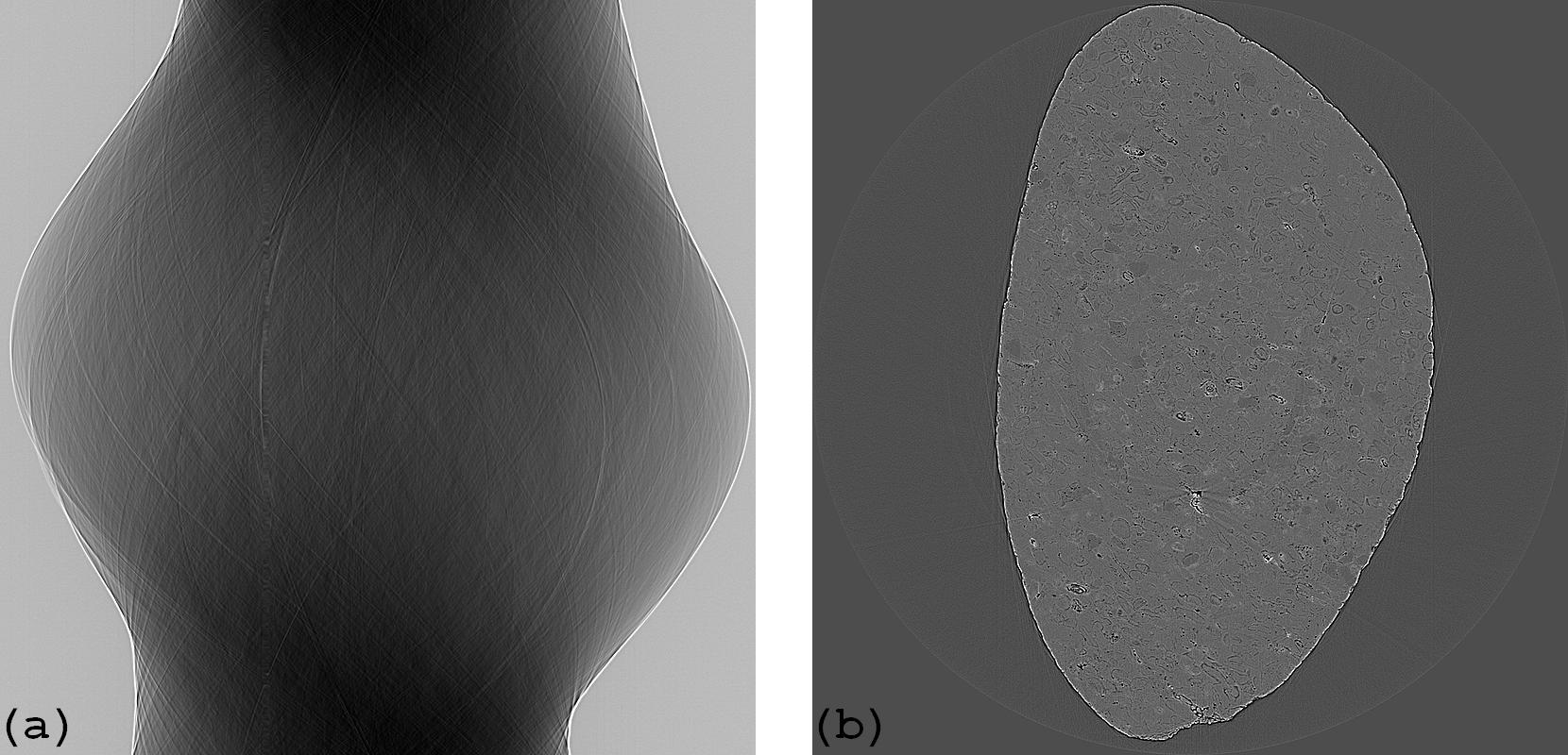
Figure 7. (a) Corrected sinogram. (b) Reconstructed image from sinogram (a).
How to use
– The snr parameter controls the sensitivity of the stripe detection method. Smaller is more sensitive. Recommended values: 1.1 -> 3.0.
– The size parameter controls the strength of the median filter and can be determined in a straightforward way by the size of dead pixels.